Compute the Sample Mean and Sample Median for Y 0y 0 Compute Them Both Again for Y 10y 10

Middle quantile of a information prepare or probability distribution

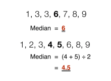
Finding the median in sets of information with an odd and even number of values

In statistics and probability theory, the median is the value separating the higher half from the lower one-half of a information sample, a population, or a probability distribution. For a information set, it may exist thought of every bit "the middle" value. The basic feature of the median in describing information compared to the mean (often just described every bit the "average") is that it is not skewed by a small proportion of extremely big or small values, and therefore provides a amend representation of a "typical" value. Median income, for case, may be a better way to advise what a "typical" income is, because income distribution can be very skewed. The median is of fundamental importance in robust statistics, as it is the near resistant statistic, having a breakup point of 50%: so long every bit no more half the data are contaminated, the median is not an arbitrarily large or small result.

Finite information set of numbers [edit]

The median of a finite list of numbers is the "heart" number, when those numbers are listed in lodge from smallest to greatest.

If the information fix has an odd number of observations, the eye i is selected. For example, the following listing of seven numbers,

1, 3, three, half dozen, 7, 8, 9

has the median of six, which is the fourth value.

If the information ready has an even number of observations, there is no distinct middle value and the median is usually divers to be the arithmetic mean of the two eye values.^{[1] [2]} For example, this data ready of viii numbers

ane, 2, 3, iv, 5, half-dozen, 8, nine

has a median value of 4.5, that is ${\displaystyle (iv+5)/2}$ . (In more than technical terms, this interprets the median as the fully trimmed mid-range).

In general, with this convention, the median tin can be divers equally follows: For a data set ${\displaystyle x}$ of ${\displaystyle n}$ elements, ordered from smallest to greatest,

if ${\displaystyle n}$ is odd, ${\displaystyle \mathrm {median} (x)=x_{(northward+i)/2}}$

if ${\displaystyle due north}$ is even, ${\displaystyle \mathrm {median} (ten)={\frac {x_{(n/2)}+x_{(n/2)+1}}{2}}}$

Comparison of mutual averages of values [ 1, ii, 2, 3, four, seven, 9 ]

Blazon	Description	Example	Result
Arithmetic mean	Sum of values of a data set divided by number of values: ${\textstyle {\bar {ten}}={\frac {ane}{n}}\sum _{i=1}^{north}x_{i}}$	(i + two + 2 + 3 + 4 + 7 + 9) / 7	4
Median	Heart value separating the greater and lesser halves of a information set	one, 2, ii, 3, iv, 7, ix	iii
Style	Most frequent value in a data set up	i, 2, 2, 3, 4, vii, 9	2

Formal definition [edit]

Formally, a median of a population is any value such that at nigh half of the population is less than the proposed median and at most half is greater than the proposed median. As seen in a higher place, medians may not be unique. If each ready contains less than half the population, then some of the population is exactly equal to the unique median.

The median is well-divers for any ordered (i-dimensional) information, and is independent of whatever distance metric. The median tin thus exist applied to classes which are ranked but not numerical (due east.chiliad. working out a median class when students are graded from A to F), although the effect might be halfway between classes if there is an fifty-fifty number of cases.

A geometric median, on the other hand, is divers in any number of dimensions. A related concept, in which the result is forced to correspond to a member of the sample, is the medoid.

There is no widely accepted standard notation for the median, but some authors represent the median of a variable ten either as x͂ or every bit μ _ane/2 ^[1] sometimes as well M.^{[3] [4]} In any of these cases, the employ of these or other symbols for the median needs to exist explicitly divers when they are introduced.

The median is a special example of other ways of summarizing the typical values associated with a statistical distribution: it is the 2nd quartile, 5th decile, and 50th percentile.

Uses [edit]

The median can be used every bit a mensurate of location when ane attaches reduced importance to extreme values, typically because a distribution is skewed, farthermost values are not known, or outliers are untrustworthy, i.eastward., may be measurement/transcription errors.

For example, consider the multiset

1, 2, 2, 2, three, fourteen.

The median is 2 in this instance, (as is the mode), and information technology might exist seen as a ameliorate indication of the middle than the arithmetic hateful of 4, which is larger than all-just-one of the values. However, the widely cited empirical relationship that the mean is shifted "further into the tail" of a distribution than the median is not generally true. At almost, one tin say that the 2 statistics cannot be "likewise far" apart; come across § Inequality relating ways and medians below.^[v]

Equally a median is based on the middle data in a set up, it is non necessary to know the value of extreme results in order to calculate it. For example, in a psychology examination investigating the fourth dimension needed to solve a problem, if a small number of people failed to solve the problem at all in the given time a median can still be calculated.^[6]

Because the median is uncomplicated to understand and easy to calculate, while likewise a robust approximation to the hateful, the median is a popular summary statistic in descriptive statistics. In this context, in that location are several choices for a measure of variability: the range, the interquartile range, the mean absolute deviation, and the median absolute deviation.

For practical purposes, unlike measures of location and dispersion are often compared on the basis of how well the corresponding population values can be estimated from a sample of data. The median, estimated using the sample median, has good properties in this regard. While information technology is not usually optimal if a given population distribution is causeless, its properties are always reasonably expert. For example, a comparing of the efficiency of candidate estimators shows that the sample hateful is more statistically efficient when — and but when — data is uncontaminated past data from heavy-tailed distributions or from mixtures of distributions.^{[ commendation needed ]} Even and so, the median has a 64% efficiency compared to the minimum-variance hateful (for large normal samples), which is to say the variance of the median volition be ~50% greater than the variance of the mean.^{[vii] [8]}

Probability distributions [edit]

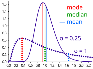
Geometric visualization of the mode, median and mean of an arbitrary probability density part^[9]

For whatever real-valued probability distribution with cumulative distribution functionF, a median is defined as any existent number1000 that satisfies the inequalities

$${\displaystyle \int _{(-\infty ,grand]}dF(10)\geq {\frac {ane}{2}}{\text{ and }}\int _{[grand,\infty )}dF(10)\geq {\frac {1}{2}}.}$$

An equivalent phrasing uses a random variable Ten distributed co-ordinate to F:

$${\displaystyle \operatorname {P} (X\leq one thousand)\geq {\frac {i}{two}}{\text{ and }}\operatorname {P} (10\geq m)\geq {\frac {1}{2}}}$$

Note that this definition does not require X to have an absolutely continuous distribution (which has a probability density function f), nor does information technology require a detached one. In the former instance, the inequalities can be upgraded to equality: a median satisfies

$${\displaystyle \operatorname {P} (X\leq chiliad)=\int _{-\infty }^{1000}{f(x)\,dx}={\frac {1}{two}}=\int _{m}^{\infty }{f(x)\,dx}=\operatorname {P} (X\geq 1000).}$$

Whatever probability distribution on R has at least ane median, but in pathological cases there may be more than one median: if F is abiding 1/2 on an interval (so that f=0 there), and then any value of that interval is a median.

Medians of particular distributions [edit]

The medians of certain types of distributions tin exist hands calculated from their parameters; furthermore, they exist even for some distributions lacking a well-defined hateful, such as the Cauchy distribution:

• The median of a symmetric unimodal distribution coincides with the mode.
• The median of a symmetric distribution which possesses a mean μ also takes the value μ.
  • The median of a normal distribution with hateful μ and variance σ ⁱⁱ is μ. In fact, for a normal distribution, hateful = median = way.
  • The median of a uniform distribution in the interval [a,b] is (a +b) / 2, which is also the mean.
• The median of a Cauchy distribution with location parameter x ₀ and scale parameter y isx ₀, the location parameter.
• The median of a power law distribution x ^−a , with exponent a > i is 2^{1/(a − 1)} x _min, where x _min is the minimum value for which the power law holds^[ten]
• The median of an exponential distribution with charge per unit parameter λ is the natural logarithm of 2 divided by the rate parameter: λ ⁻¹ln 2.
• The median of a Weibull distribution with shape parameter k and scale parameter λ isλ(ln 2)^one/k .

Populations [edit]

Optimality belongings [edit]

The mean absolute error of a existent variable c with respect to the random variableX is

${\displaystyle Due east(\left|Ten-c\right|)\,}$

Provided that the probability distribution of X is such that the in a higher place expectation exists, then 1000 is a median of X if and simply if grand is a minimizer of the mean accented mistake with respect to X.^[11] In particular, m is a sample median if and simply if m minimizes the arithmetic mean of the absolute deviations.^[12]

More generally, a median is defined as a minimum of

${\displaystyle E(|X-c|-|Ten|),}$

as discussed below in the department on multivariate medians (specifically, the spatial median).

This optimization-based definition of the median is useful in statistical information-analysis, for example, in yard-medians clustering.

Inequality relating means and medians [edit]

If the distribution has finite variance, then the distance between the median ${\displaystyle {\tilde {X}}}$ and the mean ${\displaystyle {\bar {X}}}$ is divisional by one standard deviation.

This jump was proved by Book and Sher in 1979 for discrete samples,^[xiii] and more than generally by Page and Murty in 1982.^[14] In a comment on a subsequent proof past O'Cinneide,^[15] Mallows in 1991 presented a compact proof that uses Jensen'south inequality twice,^[16] as follows. Using |·| for the absolute value, we have

${\displaystyle {\brainstorm{aligned}|\mu -grand|=|\operatorname {E} (Ten-m)|&\leq \operatorname {Eastward} (|10-chiliad|)\\&\leq \operatorname {E} (|X-\mu |)\\&\leq {\sqrt {\operatorname {E} \left((X-\mu )^{2}\right)}}=\sigma .\terminate{aligned}}}$

The kickoff and third inequalities come from Jensen's inequality applied to the absolute-value function and the square function, which are each convex. The 2nd inequality comes from the fact that a median minimizes the absolute deviation function ${\displaystyle a\mapsto \operatorname {Eastward} (|X-a|)}$ .

Mallows' proof can be generalized to obtain a multivariate version of the inequality^[17] simply by replacing the absolute value with a norm:

${\displaystyle \|\mu -m\|\leq {\sqrt {\operatorname {E} \left(\|X-\mu \|^{ii}\right)}}={\sqrt {\operatorname {trace} \left(\operatorname {var} (X)\correct)}}}$

where yard is a spatial median, that is, a minimizer of the function ${\displaystyle a\mapsto \operatorname {Eastward} (\|X-a\|).\,}$ The spatial median is unique when the information-ready's dimension is two or more.^{[18] [xix]}

An alternative proof uses the i-sided Chebyshev inequality; information technology appears in an inequality on location and calibration parameters. This formula also follows directly from Cantelli's inequality.^[20]

Unimodal distributions [edit]

For the instance of unimodal distributions, one can accomplish a sharper bound on the distance between the median and the mean:

${\displaystyle \left|{\tilde {X}}-{\bar {Ten}}\right|\leq \left({\frac {3}{5}}\correct)^{\frac {1}{ii}}\sigma \approx 0.7746\sigma }$ .^[21]

A like relation holds between the median and the style:

${\displaystyle \left|{\tilde {10}}-\mathrm {mode} \right|\leq 3^{\frac {1}{ii}}\sigma \approx 1.732\sigma .}$

Jensen's inequality for medians [edit]

Jensen'due south inequality states that for any random variable Ten with a finite expectation E[Ten] and for any convex function f

${\displaystyle f[E(ten)]\leq E[f(ten)]}$

This inequality generalizes to the median besides. We say a role f: R → R is a C function if, for any t,

${\displaystyle f^{-i}\left(\,(-\infty ,t]\,\right)=\{ten\in \mathbb {R} \mid f(x)\leq t\}}$

is a closed interval (assuasive the degenerate cases of a single point or an empty ready). Every convex function is a C role, but the reverse does non hold. If f is a C role, and then

${\displaystyle f(\operatorname {Median} [X])\leq \operatorname {Median} [f(X)]}$

If the medians are not unique, the argument holds for the corresponding suprema.^[22]

Medians for samples [edit]

This section discusses the theory of estimating a population median from a sample. To calculate the median of a sample "by hand," see § Finite data set up of numbers above.

The sample median [edit]

Efficient computation of the sample median [edit]

Fifty-fifty though comparing-sorting n items requires Ω(northward log northward) operations, selection algorithms tin compute the grandth-smallest of due north items with just Θ(northward) operations. This includes the median, which is the due north / two thursday order statistic (or for an even number of samples, the arithmetics mean of the two middle guild statistics).^[23]

Pick algorithms still have the downside of requiring Ω(n) memory, that is, they need to have the full sample (or a linear-sized portion of it) in memory. Considering this, as well as the linear time requirement, can exist prohibitive, several estimation procedures for the median have been developed. A simple one is the median of three rule, which estimates the median as the median of a iii-element subsample; this is commonly used equally a subroutine in the quicksort sorting algorithm, which uses an estimate of its input'southward median. A more than robust estimator is Tukey's ninther, which is the median of three dominion applied with limited recursion:^[24] if A is the sample laid out as an assortment, and

med3(A) = median(A[one], A[ due north / two ], A[due north]),

and so

ninther(A) = med3(med3(A[ane ... one / 3 n]), med3(A[ 1 / three n ... 2 / 3 n]), med3(A[ two / 3 due north ... north]))

The remedian is an estimator for the median that requires linear time simply sub-linear retentiveness, operating in a single laissez passer over the sample.^[25]

Sampling distribution [edit]

The distributions of both the sample mean and the sample median were adamant by Laplace.^[26] The distribution of the sample median from a population with a density function ${\displaystyle f(x)}$ is asymptotically normal with hateful ${\displaystyle m}$ and variance^[27]

${\displaystyle {\frac {1}{4nf(m)^{2}}}}$

where ${\displaystyle 1000}$ is the median of ${\displaystyle f(10)}$ and ${\displaystyle n}$ is the sample size. A mod proof follows below. Laplace'south result is at present understood as a special case of the asymptotic distribution of arbitrary quantiles.

For normal samples, the density is ${\displaystyle f(m)=i/{\sqrt {two\pi \sigma ^{ii}}}}$ , thus for big samples the variance of the median equals ${\displaystyle ({\pi }/{2})\cdot (\sigma ^{2}/n).}$ ^[7] (Run across too section #Efficiency below.)

Derivation of the asymptotic distribution [edit]

We take the sample size to be an odd number ${\displaystyle N=2n+1}$ and assume our variable continuous; the formula for the instance of discrete variables is given below in § Empirical local density. The sample tin be summarized equally "beneath median", "at median", and "above median", which corresponds to a trinomial distribution with probabilities ${\displaystyle F(v-1)}$ , ${\displaystyle f(five)}$ and ${\displaystyle i-F(5)}$ . For a continuous variable, the probability of multiple sample values being exactly equal to the median is 0, and so one can calculate the density of at the point ${\displaystyle v}$ direct from the trinomial distribution:

${\displaystyle \Pr[\operatorname {Median} =v]\,dv={\frac {(2n+one)!}{due north!north!}}F(v)^{north}(1-F(5))^{n}f(v)\,dv}$ .

Now we introduce the beta role. For integer arguments ${\displaystyle \alpha }$ and ${\displaystyle \beta }$ , this can be expressed as ${\displaystyle \mathrm {B} (\alpha ,\beta )={\frac {(\alpha -1)!(\beta -1)!}{(\alpha +\beta -one)!}}}$ . Also, recall that ${\displaystyle f(5)\,dv=dF(five)}$ . Using these relationships and setting both ${\displaystyle \alpha }$ and ${\displaystyle \beta }$ equal to ${\displaystyle n+i}$ allows the final expression to be written equally

${\displaystyle {\frac {F(v)^{n}(i-F(v))^{due north}}{\mathrm {B} (north+ane,n+1)}}\,dF(v)}$

Hence the density part of the median is a symmetric beta distribution pushed frontward by ${\displaystyle F}$ . Its mean, every bit we would look, is 0.5 and its variance is ${\displaystyle 1/(4(North+2))}$ . By the concatenation dominion, the respective variance of the sample median is

${\displaystyle {\frac {1}{4(N+2)f(m)^{2}}}}$ .

The boosted ii is negligible in the limit.

Empirical local density [edit]

In do, the functions ${\displaystyle f}$ and ${\displaystyle F}$ are often not known or assumed. However, they can be estimated from an observed frequency distribution. In this section, nosotros give an example. Consider the following table, representing a sample of three,800 (detached-valued) observations:

v	0	0.5	1	ane.5	2	2.5	3	3.5	4	four.5	five
f(v)	0.000	0.008	0.010	0.013	0.083	0.108	0.328	0.220	0.202	0.023	0.005
F(v)	0.000	0.008	0.018	0.031	0.114	0.222	0.550	0.770	0.972	0.995	one.000

Considering the observations are discrete-valued, amalgam the exact distribution of the median is not an immediate translation of the higher up expression for ${\displaystyle \Pr(\operatorname {Median} =v)}$ ; 1 may (and typically does) have multiple instances of the median in one's sample. So nosotros must sum over all these possibilities:

${\displaystyle \Pr(\operatorname {Median} =v)=\sum _{i=0}^{n}\sum _{k=0}^{n}{\frac {N!}{i!(Due north-i-1000)!k!}}F(v-one)^{i}(1-F(v))^{thousand}f(five)^{N-i-k}}$

Here, i is the number of points strictly less than the median and one thousand the number strictly greater.

Using these preliminaries, it is possible to investigate the effect of sample size on the standard errors of the mean and median. The observed hateful is 3.16, the observed raw median is 3 and the observed interpolated median is 3.174. The post-obit table gives some comparison statistics.

Sample size Statistic	3	9	xv	21
Expected value of median	3.198	3.191	3.174	three.161
Standard fault of median (to a higher place formula)	0.482	0.305	0.257	0.239
Standard fault of median (asymptotic approximation)	0.879	0.508	0.393	0.332
Standard mistake of hateful	0.421	0.243	0.188	0.159

The expected value of the median falls slightly equally sample size increases while, as would be expected, the standard errors of both the median and the mean are proportionate to the inverse foursquare root of the sample size. The asymptotic approximation errs on the side of caution past overestimating the standard error.

Estimation of variance from sample data [edit]

The value of ${\displaystyle (2f(x))^{-2}}$ —the asymptotic value of ${\displaystyle northward^{-{\frac {i}{2}}}(\nu -yard)}$ where ${\displaystyle \nu }$ is the population median—has been studied by several authors. The standard "delete one" jackknife method produces inconsistent results.^[28] An alternative—the "delete k" method—where ${\displaystyle k}$ grows with the sample size has been shown to be asymptotically consistent.^[29] This method may be computationally expensive for big information sets. A bootstrap approximate is known to be consistent,^[30] merely converges very slowly (order of ${\displaystyle n^{-{\frac {one}{4}}}}$ ).^[31] Other methods accept been proposed but their behavior may differ between big and small samples.^[32]

Efficiency [edit]

The efficiency of the sample median, measured as the ratio of the variance of the hateful to the variance of the median, depends on the sample size and on the underlying population distribution. For a sample of size ${\displaystyle N=2n+1}$ from the normal distribution, the efficiency for big Due north is

${\displaystyle {\frac {2}{\pi }}{\frac {N+ii}{N}}}$

The efficiency tends to ${\displaystyle {\frac {2}{\pi }}}$ as ${\displaystyle N}$ tends to infinity.

In other words, the relative variance of the median will exist ${\displaystyle \pi /two\approx 1.57}$ , or 57% greater than the variance of the mean – the relative standard error of the median will be ${\displaystyle (\pi /2)^{\frac {1}{2}}\approx one.25}$ , or 25% greater than the standard error of the mean, ${\displaystyle \sigma /{\sqrt {north}}}$ (see too section #Sampling distribution above.).^[33]

Other estimators [edit]

For univariate distributions that are symmetric almost one median, the Hodges–Lehmann computer is a robust and highly efficient estimator of the population median.^[34]

If data is represented past a statistical model specifying a detail family of probability distributions, then estimates of the median can be obtained past plumbing equipment that family of probability distributions to the data and calculating the theoretical median of the fitted distribution.^{[ citation needed ]} Pareto interpolation is an application of this when the population is assumed to have a Pareto distribution.

Multivariate median [edit]

Previously, this article discussed the univariate median, when the sample or population had one-dimension. When the dimension is two or college, there are multiple concepts that extend the definition of the univariate median; each such multivariate median agrees with the univariate median when the dimension is exactly one.^{[34] [35] [36] [37]}

Marginal median [edit]

The marginal median is defined for vectors defined with respect to a fixed gear up of coordinates. A marginal median is defined to be the vector whose components are univariate medians. The marginal median is easy to compute, and its properties were studied by Puri and Sen.^{[34] [38]}

Geometric median [edit]

The geometric median of a discrete set of sample points ${\displaystyle x_{one},\ldots x_{Due north}}$ in a Euclidean space is the^[a] point minimizing the sum of distances to the sample points.

${\displaystyle {\hat {\mu }}={\underset {\mu \in \mathbb {R} ^{g}}{\operatorname {arg\,min} }}\sum _{n=1}^{N}\left\|\mu -x_{n}\right\|_{2}}$

In contrast to the marginal median, the geometric median is equivariant with respect to Euclidean similarity transformations such as translations and rotations.

Median in all directions [edit]

If the marginal medians for all coordinate systems coincide, then their common location may exist termed the "median in all directions".^[xl] This concept is relevant to voting theory on account of the median voter theorem. When information technology exists, the median in all directions coincides with the geometric median (at to the lowest degree for discrete distributions).

Centerpoint [edit]

An culling generalization of the median in college dimensions is the centerpoint.

[edit]

Interpolated median [edit]

When dealing with a discrete variable, it is sometimes useful to regard the observed values as beingness midpoints of underlying continuous intervals. An example of this is a Likert calibration, on which opinions or preferences are expressed on a scale with a set number of possible responses. If the scale consists of the positive integers, an observation of 3 might exist regarded as representing the interval from two.50 to iii.l. Information technology is possible to judge the median of the underlying variable. If, say, 22% of the observations are of value two or below and 55.0% are of 3 or below (so 33% have the value 3), so the median ${\displaystyle m}$ is 3 since the median is the smallest value of ${\displaystyle x}$ for which ${\displaystyle F(10)}$ is greater than a half. But the interpolated median is somewhere between 2.50 and iii.50. First we add one-half of the interval width ${\displaystyle w}$ to the median to get the upper bound of the median interval. Then we subtract that proportion of the interval width which equals the proportion of the 33% which lies higher up the l% mark. In other words, we split up the interval width pro rata to the numbers of observations. In this case, the 33% is divide into 28% below the median and 5% above it so we subtract 5/33 of the interval width from the upper bound of 3.l to give an interpolated median of iii.35. More formally, if the values ${\displaystyle f(x)}$ are known, the interpolated median tin can be calculated from

${\displaystyle m_{\text{int}}=m+w\left[{\frac {one}{2}}-{\frac {F(g)-{\frac {1}{ii}}}{f(chiliad)}}\right].}$

Alternatively, if in an observed sample there are ${\displaystyle yard}$ scores above the median category, ${\displaystyle j}$ scores in it and ${\displaystyle i}$ scores below information technology so the interpolated median is given by

${\displaystyle m_{\text{int}}=m-{\frac {w}{2}}\left[{\frac {m-i}{j}}\correct].}$

Pseudo-median [edit]

For univariate distributions that are symmetric about one median, the Hodges–Lehmann figurer is a robust and highly efficient reckoner of the population median; for non-symmetric distributions, the Hodges–Lehmann estimator is a robust and highly efficient estimator of the population pseudo-median, which is the median of a symmetrized distribution and which is shut to the population median.^[41] The Hodges–Lehmann estimator has been generalized to multivariate distributions.^[42]

Variants of regression [edit]

The Theil–Sen estimator is a method for robust linear regression based on finding medians of slopes.^[43]

Median filter [edit]

The median filter is an important tool of image processing, that can effectively remove whatever common salt and pepper dissonance from grayscale images.

Cluster assay [edit]

In cluster assay, the thousand-medians clustering algorithm provides a fashion of defining clusters, in which the criterion of maximising the distance between cluster-ways that is used in k-means clustering, is replaced by maximising the altitude between cluster-medians.

Median–median line [edit]

This is a method of robust regression. The idea dates back to Wald in 1940 who suggested dividing a set of bivariate data into ii halves depending on the value of the independent parameter ${\displaystyle x}$ : a left half with values less than the median and a right half with values greater than the median.^[44] He suggested taking the means of the dependent ${\displaystyle y}$ and contained ${\displaystyle 10}$ variables of the left and the right halves and estimating the gradient of the line joining these two points. The line could then be adjusted to fit the majority of the points in the data set.

Nair and Shrivastava in 1942 suggested a similar idea but instead advocated dividing the sample into 3 equal parts before calculating the means of the subsamples.^[45] Brown and Mood in 1951 proposed the idea of using the medians of two subsamples rather the means.^[46] Tukey combined these ideas and recommended dividing the sample into three equal size subsamples and estimating the line based on the medians of the subsamples.^[47]

Median-unbiased estimators [edit]

Whatever mean-unbiased estimator minimizes the risk (expected loss) with respect to the squared-error loss office, every bit observed by Gauss. A median-unbiased estimator minimizes the risk with respect to the absolute-deviation loss function, as observed by Laplace. Other loss functions are used in statistical theory, particularly in robust statistics.

The theory of median-unbiased estimators was revived by George West. Chocolate-brown in 1947:^[48]

An guess of a one-dimensional parameter θ will be said to be median-unbiased if, for fixed θ, the median of the distribution of the gauge is at the value θ; i.due east., the approximate underestimates just equally often equally it overestimates. This requirement seems for most purposes to accomplish equally much as the hateful-unbiased requirement and has the additional property that it is invariant under one-to-1 transformation.

—page 584

Further backdrop of median-unbiased estimators have been reported.^{[49] [l] [51] [52]} Median-unbiased estimators are invariant under ane-to-one transformations.

There are methods of constructing median-unbiased estimators that are optimal (in a sense analogous to the minimum-variance property for mean-unbiased estimators). Such constructions exist for probability distributions having monotone likelihood-functions.^{[53] [54]} One such procedure is an analogue of the Rao–Blackwell procedure for hateful-unbiased estimators: The procedure holds for a smaller form of probability distributions than does the Rao—Blackwell procedure but for a larger class of loss functions.^[55]

History [edit]

Scientific researchers in the aboriginal virtually eastward appear not to accept used summary statistics altogether, instead choosing values that offered maximal consistency with a broader theory that integrated a broad multifariousness of phenomena.^[56] Inside the Mediterranean (and, later, European) scholarly community, statistics like the mean are fundamentally a medieval and early modern development. (The history of the median outside Europe and its predecessors remains relatively unstudied.)

The idea of the median appeared in the sixth century in the Talmud, in gild to fairly analyze divergent appraisals.^{[57] [58]} Nevertheless, the concept did not spread to the broader scientific customs.

Instead, the closest ancestor of the modern median is the mid-range, invented by Al-Biruni.^{[59] : 31 [60]} Transmission of Al-Biruni's work to after scholars is unclear. Al-Biruni practical his technique to assaying metals, but, later he published his work, nigh assayers even so adopted the most unfavorable value from their results, lest they appear to cheat.^{[59] : 35–8} However, increased navigation at sea during the Historic period of Discovery meant that ship'due south navigators increasingly had to attempt to make up one's mind latitude in unfavorable weather against hostile shores, leading to renewed interest in summary statistics. Whether rediscovered or independently invented, the mid-range is recommended to nautical navigators in Harriot'due south "Instructions for Raleigh's Voyage to Guiana, 1595".^{[59] : 45–8}

The idea of the median may have first appeared in Edward Wright's 1599 volume Certaine Errors in Navigation on a section most compass navigation. Wright was reluctant to discard measured values, and may have felt that the median — incorporating a greater proportion of the dataset than the mid-range — was more than likely to be correct. However, Wright did not give examples of his technique'south use, making it hard to verify that he described the modern notion of median.^{[56] [60] [b]} The median (in the context of probability) certainly appeared in the correspondence of Christiaan Huygens, but as an example of a statistic that was inappropriate for actuarial do.^[56]

The earliest recommendation of the median dates to 1757, when Roger Joseph Boscovich developed a regression method based on the L ¹ norm and therefore implicitly on the median.^{[56] [61]} In 1774, Laplace made this desire explicit: he suggested the median be used as the standard figurer of the value of a posterior PDF. The specific benchmark was to minimize the expected magnitude of the error; ${\displaystyle |\blastoff -\alpha ^{*}|}$ where ${\displaystyle \alpha ^{*}}$ is the estimate and ${\displaystyle \alpha }$ is the truthful value. To this end, Laplace determined the distributions of both the sample mean and the sample median in the early 1800s.^{[26] [62]} However, a decade later, Gauss and Legendre developed the least squares method, which minimizes ${\displaystyle (\alpha -\alpha ^{*})^{2}}$ to obtain the mean. Within the context of regression, Gauss and Legendre'south innovation offers vastly easier computation. Consequently, Laplaces' proposal was by and large rejected until the ascent of calculating devices 150 years after (and is still a relatively uncommon algorithm).^[63]

Antoine Augustin Cournot in 1843 was the first^[64] to use the term median (valeur médiane) for the value that divides a probability distribution into 2 equal halves. Gustav Theodor Fechner used the median (Centralwerth) in sociological and psychological phenomena.^[65] Information technology had earlier been used only in astronomy and related fields. Gustav Fechner popularized the median into the formal analysis of data, although it had been used previously by Laplace,^[65] and the median appeared in a textbook by F. Y. Edgeworth.^[66] Francis Galton used the English term median in 1881,^{[67] [68]} having before used the terms center-well-nigh value in 1869, and the medium in 1880.^{[69] [70]}

Statisticians encouraged the use of medians intensely throughout the 19th century for its intuitive clarity and ease of manual computation. Notwithstanding, the notion of median does not lend itself to the theory of higher moments as well as the arithmetics mean does, and is much harder to compute by figurer. As a result, the median was steadily supplanted equally a notion of generic average by the arithmetics mean during the 20th century.^{[56] [lx]}

See besides [edit]

• Medoids which are a generalisation of the median in higher dimensions
• Key trend
  • Hateful
  • Mode
• Absolute deviation
• Bias of an calculator
• Concentration of measure out for Lipschitz functions
• Median (geometry)
• Median graph
• Median search
• Median slope
• Median voter theory
• Weighted median
• Median of medians: Algorithm to summate the approximate median in linear fourth dimension
• Order statistic

Notes [edit]

1. ^ The geometric median is unique unless the sample is collinear.^[39]
2. ^ Subsequent scholars appear to concur with Eisenhart that Boroughs' 1580 figures, while suggestive of the median, in fact describe an arithmetics mean.;^{[59] : 62–iii} Boroughs is mentioned in no other work.

References [edit]

1. ^ ^{a b} Weisstein, Eric W. "Statistical Median". MathWorld.
2. ^ Simon, Laura J.; "Descriptive statistics" Archived 2010-07-30 at the Wayback Machine, Statistical Education Resource Kit, Pennsylvania Land Department of Statistics
3. ^ David J. Sheskin (27 August 2003). Handbook of Parametric and Nonparametric Statistical Procedures (Third ed.). CRC Press. pp. 7–. ISBN978-one-4200-3626-8 . Retrieved 25 February 2013.
4. ^ Derek Bissell (1994). Statistical Methods for Spc and Tqm. CRC Printing. pp. 26–. ISBN978-0-412-39440-9 . Retrieved 25 February 2013.
5. ^ Paul T. von Hippel (2005). "Mean, Median, and Skew: Correcting a Textbook Dominion". Periodical of Statistics Education. thirteen (2).
6. ^ Robson, Colin (1994). Experiment, Design and Statistics in Psychology. Penguin. pp. 42–45. ISBN0-14-017648-9.
7. ^ ^{a b} Williams, D. (2001). Weighing the Odds . Cambridge University Press. p. 165. ISBN052100618X.
8. ^ Maindonald, John; Braun, W. John (2010-05-06). Data Analysis and Graphics Using R: An Example-Based Approach. Cambridge University Press. p. 104. ISBN978-1-139-48667-5.
9. ^ "AP Statistics Review - Density Curves and the Normal Distributions". Archived from the original on 8 April 2015. Retrieved 16 March 2015.
10. ^ Newman, Mark EJ. "Power laws, Pareto distributions and Zipf's law." Contemporary physics 46.5 (2005): 323–351.
11. ^ Stroock, Daniel (2011). Probability Theory . Cambridge University Printing. pp. 43. ISBN978-0-521-13250-three.
12. ^ André Nicolas (https://math.stackexchange.com/users/6312/andr%c3%a9-nicolas), The Median Minimizes the Sum of Absolute Deviations (The $ {L}_{one} $ Norm), URL (version: 2012-02-25): https://math.stackexchange.com/q/113336
13. ^ Stephen A. Book; Lawrence Sher (1979). "How close are the mean and the median?". The Two-Year College Mathematics Journal. x (iii): 202–204. doi:10.2307/3026748. JSTOR 3026748. Retrieved 12 March 2022.
14. ^ Warren Page; Vedula North. Murty (1982). "Nearness Relations Amidst Measures of Central Trend and Dispersion: Part 1". The 2-Twelvemonth College Mathematics Periodical. 13 (5): 315–327. doi:10.1080/00494925.1982.11972639 (inactive 2022-04-xix). Retrieved 12 March 2022. {{cite journal}}: CS1 maint: DOI inactive equally of April 2022 (link)
15. ^ O'Cinneide, Colm Art (1990). "The mean is inside one standard deviation of any median". The American Statistician. 44 (iv): 292–293. doi:10.1080/00031305.1990.10475743. Retrieved 12 March 2022.
16. ^ Mallows, Colin (August 1991). "Another comment on O'Cinneide". The American Statistician. 45 (three): 257. doi:10.1080/00031305.1991.10475815.
17. ^ Piché, Robert (2012). Random Vectors and Random Sequences. Lambert Academic Publishing. ISBN978-3659211966.
18. ^ Kemperman, Johannes H. B. (1987). Contrivance, Yadolah (ed.). "The median of a finite measure on a Banach space: Statistical information analysis based on the L1-norm and related methods". Papers from the First International Conference Held at Neuchâtel, August 31–September 4, 1987. Amsterdam: N-Holland Publishing Co.: 217–230. MR 0949228.
19. ^ Milasevic, Philip; Ducharme, Gilles R. (1987). "Uniqueness of the spatial median". Annals of Statistics. fifteen (three): 1332–1333. doi:10.1214/aos/1176350511. MR 0902264.
20. ^ K.Van Steen Notes on probability and statistics
21. ^ Basu, S.; Dasgupta, A. (1997). "The Mean, Median, and Manner of Unimodal Distributions:A Characterization". Theory of Probability and Its Applications. 41 (ii): 210–223. doi:x.1137/S0040585X97975447. S2CID 54593178.
22. ^ Merkle, M. (2005). "Jensen's inequality for medians". Statistics & Probability Letters. 71 (3): 277–281. doi:x.1016/j.spl.2004.11.010.
23. ^ Alfred V. Aho and John Due east. Hopcroft and Jeffrey D. Ullman (1974). The Design and Analysis of Computer Algorithms . Reading/MA: Addison-Wesley. ISBN0-201-00029-6. Hither: Section 3.vi "Order Statistics", p.97-99, in particular Algorithm 3.half dozen and Theorem iii.nine.
24. ^ Bentley, Jon L.; McIlroy, Grand. Douglas (1993). "Engineering a sort function". Software: Practice and Experience. 23 (eleven): 1249–1265. doi:10.1002/spe.4380231105. S2CID 8822797.
25. ^ Rousseeuw, Peter J.; Bassett, Gilbert West. Jr. (1990). "The remedian: a robust averaging method for large data sets" (PDF). J. Amer. Statist. Assoc. 85 (409): 97–104. doi:ten.1080/01621459.1990.10475311.
26. ^ ^{a b} Stigler, Stephen (December 1973). "Studies in the History of Probability and Statistics. XXXII: Laplace, Fisher and the Discovery of the Concept of Sufficiency". Biometrika. threescore (three): 439–445. doi:10.1093/biomet/lx.iii.439. JSTOR 2334992. MR 0326872.
27. ^ Rider, Paul R. (1960). "Variance of the median of small samples from several special populations". J. Amer. Statist. Assoc. 55 (289): 148–150. doi:10.1080/01621459.1960.10482056.
28. ^ Efron, B. (1982). The Jackknife, the Bootstrap and other Resampling Plans. Philadelphia: SIAM. ISBN0898711797.
29. ^ Shao, J.; Wu, C. F. (1989). "A Full general Theory for Jackknife Variance Estimation". Ann. Stat. 17 (3): 1176–1197. doi:10.1214/aos/1176347263. JSTOR 2241717.
30. ^ Efron, B. (1979). "Bootstrap Methods: Another Look at the Jackknife". Ann. Stat. seven (1): i–26. doi:x.1214/aos/1176344552. JSTOR 2958830.
31. ^ Hall, P.; Martin, M. A. (1988). "Exact Convergence Rate of Bootstrap Quantile Variance Computer". Probab Theory Related Fields. lxxx (2): 261–268. doi:10.1007/BF00356105. S2CID 119701556.
32. ^ Jiménez-Gamero, M. D.; Munoz-García, J.; Pino-Mejías, R. (2004). "Reduced bootstrap for the median". Statistica Sinica. 14 (4): 1179–1198.
33. ^ Maindonald, John; John Braun, W. (2010-05-06). Data Assay and Graphics Using R: An Instance-Based Approach. ISBN9781139486675.
34. ^ ^{a b c} Hettmansperger, Thomas P.; McKean, Joseph Due west. (1998). Robust nonparametric statistical methods. Kendall'south Library of Statistics. Vol. 5. London: Edward Arnold. ISBN0-340-54937-eight. MR 1604954.
35. ^ Small, Christopher G. "A survey of multidimensional medians." International Statistical Review/Revue Internationale de Statistique (1990): 263–277. doi:ten.2307/1403809 JSTOR 1403809
36. ^ Niinimaa, A., and H. Oja. "Multivariate median." Encyclopedia of statistical sciences (1999).
37. ^ Mosler, Karl. Multivariate Dispersion, Primal Regions, and Depth: The Lift Zonoid Approach. Vol. 165. Springer Scientific discipline & Business Media, 2012.
38. ^ Puri, Madan L.; Sen, Pranab Thousand.; Nonparametric Methods in Multivariate Analysis, John Wiley & Sons, New York, NY, 1971. (Reprinted by Krieger Publishing)
39. ^ Vardi, Yehuda; Zhang, Cun-Hui (2000). "The multivariate L _i-median and associated data depth". Proceedings of the National Academy of Sciences of the United States of America. 97 (4): 1423–1426 (electronic). Bibcode:2000PNAS...97.1423V. doi:10.1073/pnas.97.4.1423. MR 1740461. PMC26449. PMID 10677477.
40. ^ Davis, Otto A.; DeGroot, Morris H.; Hinich, Melvin J. (January 1972). "Social Preference Orderings and Majority Rule" (PDF). Econometrica. 40 (1): 147–157. doi:x.2307/1909727. JSTOR 1909727. The authors, working in a topic in which uniqueness is causeless, really use the expression "unique median in all directions".
41. ^ Pratt, William Thou.; Cooper, Ted J.; Kabir, Ihtisham (1985-07-11). Corbett, Francis J (ed.). "Pseudomedian Filter". Architectures and Algorithms for Digital Paradigm Processing II. 0534: 34. Bibcode:1985SPIE..534...34P. doi:ten.1117/12.946562. S2CID 173183609.
42. ^ Oja, Hannu (2010). Multivariate nonparametric methods withR: An approach based on spatial signs and ranks. Lecture Notes in Statistics. Vol. 199. New York, NY: Springer. pp. fourteen+232. doi:x.1007/978-1-4419-0468-3. ISBN978-one-4419-0467-6. MR 2598854.
43. ^ Wilcox, Rand R. (2001), "Theil–Sen figurer", Fundamentals of Modern Statistical Methods: Substantially Improving Power and Accuracy, Springer-Verlag, pp. 207–210, ISBN978-0-387-95157-7 .
44. ^ Wald, A. (1940). "The Fitting of Straight Lines if Both Variables are Subject to Mistake" (PDF). Annals of Mathematical Statistics. 11 (3): 282–300. doi:10.1214/aoms/1177731868. JSTOR 2235677.
45. ^ Nair, Thou. R.; Shrivastava, M. P. (1942). "On a Elementary Method of Curve Fitting". Sankhyā: The Indian Journal of Statistics. half dozen (2): 121–132. JSTOR 25047749.
46. ^ Brown, G. W.; Mood, A. M. (1951). "On Median Tests for Linear Hypotheses". Proc Second Berkeley Symposium on Mathematical Statistics and Probability. Berkeley, CA: University of California Press. pp. 159–166. Zbl 0045.08606.
47. ^ Tukey, J. W. (1977). Exploratory Data Analysis. Reading, MA: Addison-Wesley. ISBN0201076160.
48. ^ Brown, George W. (1947). "On Pocket-size-Sample Interpretation". Annals of Mathematical Statistics. eighteen (four): 582–585. doi:ten.1214/aoms/1177730349. JSTOR 2236236.
49. ^ Lehmann, Erich L. (1951). "A Full general Concept of Unbiasedness". Annals of Mathematical Statistics. 22 (iv): 587–592. doi:10.1214/aoms/1177729549. JSTOR 2236928.
50. ^ Birnbaum, Allan (1961). "A Unified Theory of Estimation, I". Annals of Mathematical Statistics. 32 (1): 112–135. doi:10.1214/aoms/1177705145. JSTOR 2237612.
51. ^ van der Vaart, H. Robert (1961). "Some Extensions of the Thought of Bias". Annals of Mathematical Statistics. 32 (2): 436–447. doi:ten.1214/aoms/1177705051. JSTOR 2237754. MR 0125674.
52. ^ Pfanzagl, Johann; with the aid of R. Hamböker (1994). Parametric Statistical Theory. Walter de Gruyter. ISBNiii-11-013863-viii. MR 1291393.
53. ^ Pfanzagl, Johann. "On optimal median unbiased estimators in the presence of nuisance parameters." The Register of Statistics (1979): 187–193.
54. ^ Chocolate-brown, 50. D.; Cohen, Arthur; Strawderman, W. East. (1976). "A Consummate Form Theorem for Strict Monotone Likelihood Ratio With Applications". Ann. Statist. 4 (4): 712–722. doi:10.1214/aos/1176343543.
55. ^ Page; Brown, L. D.; Cohen, Arthur; Strawderman, W. E. (1976). "A Complete Class Theorem for Strict Monotone Likelihood Ratio With Applications". Ann. Statist. 4 (4): 712–722. doi:10.1214/aos/1176343543.
56. ^ ^{a b c d eastward} Bakker, Arthur; Gravemeijer, Koeno P. E. (2006-06-01). "An Historical Phenomenology of Mean and Median". Educational Studies in Mathematics. 62 (ii): 149–168. doi:10.1007/s10649-006-7099-8. ISSN 1573-0816. S2CID 143708116.
57. ^ Adler, Dan (31 December 2014). "Talmud and Modern Economics". Jewish American and Israeli Issues. Archived from the original on vi December 2015. Retrieved 22 February 2020.
58. ^ Modern Economic Theory in the Talmud by Yisrael Aumann
59. ^ ^{a b c d} Eisenhart, Churchill (24 August 1971). The Development of the Concept of the Best Mean of a Set of Measurements from Antiquity to the Present Day (PDF) (Speech). 131st Annual Meeting of the American Statistical Association. Colorado State University.
60. ^ ^{a b c} "How the Average Triumphed Over the Median". Priceonomics. 5 April 2016. Retrieved 2020-02-23 .
61. ^ Stigler, S. M. (1986). The History of Statistics: The Measurement of Incertitude Before 1900. Harvard University Press. ISBN0674403401.
62. ^ Laplace PS de (1818) Deuxième supplément à la Théorie Analytique des Probabilités, Paris, Courcier
63. ^ Jaynes, E.T. (2007). Probability theory : the logic of scientific discipline (5. print. ed.). Cambridge [u.a.]: Cambridge Univ. Press. p. 172. ISBN978-0-521-59271-0.
64. ^ Howarth, Richard (2017). Dictionary of Mathematical Geosciences: With Historical Notes. Springer. p. 374.
65. ^ ^{a b} Keynes, J.M. (1921) A Treatise on Probability. Pt II Ch XVII §5 (p 201) (2006 reprint, Cosimo Classics, ISBN 9781596055308 : multiple other reprints)
66. ^ Stigler, Stephen G. (2002). Statistics on the Table: The History of Statistical Concepts and Methods. Harvard University Press. pp. 105–7. ISBN978-0-674-00979-0.
67. ^ Galton F (1881) "Report of the Anthropometric Committee" pp 245–260. Written report of the 51st Coming together of the British Association for the Advancement of Science
68. ^ David, H. A. (1995). "First (?) Occurrence of Common Terms in Mathematical Statistics". The American Statistician. 49 (2): 121–133. doi:10.2307/2684625. ISSN 0003-1305. JSTOR 2684625.
69. ^ encyclopediaofmath.org
70. ^ personal.psu.edu

External links [edit]

• "Median (in statistics)", Encyclopedia of Mathematics, European monetary system Press, 2001 [1994]
• Median as a weighted arithmetic hateful of all Sample Observations
• On-line computer
• Calculating the median
• A problem involving the hateful, the median, and the manner.
• Weisstein, Eric West. "Statistical Median". MathWorld.
• Python script for Median computations and income inequality metrics
• Fast Computation of the Median by Successive Binning
• 'Mean, median, fashion and skewness', A tutorial devised for outset-yr psychology students at Oxford Academy, based on a worked instance.
• The Complex Saturday Math Trouble Even the College Board Got Incorrect: Andrew Daniels in Popular Mechanics

This article incorporates fabric from Median of a distribution on PlanetMath, which is licensed under the Artistic Commons Attribution/Share-Alike License.

campbellinever.blogspot.com

Source: https://en.wikipedia.org/wiki/Median

Share this post